pPerturb - Help

How to Use pPerturb

The pPerturb web-server provides an easy means to extract the extent to which a residue is connected to its neighbors, the functional form of its percolation, the strength of an interaction network, and to quantify the mutation-induced changes in stability. The web-server is divided into four independent modules as described below,

Generate Perturbation Profile(s): This module allows the users to simulate mutation of one or more residues to alanine and generates perturbation profiles (∆Q vs. Cα-Cα distance from the perturbed site) for select residues.
Generate Interaction-Network Profile: This module iteratively perturbs all residues in the selected protein chain and estimates the extent of percolation (coupling distance; dC) and the total magnitude of perturbation (Σ∆Q) from the individual perturbation profiles.
Compare Interaction-Network Profiles: This module allows the users to compare the interaction-network of a protein at two different states. For example, it can be used to quantify the differences in packing between ligand-bound and unbound forms of the same protein.
Predict Destabilization Thermodynamics: This module simulates the effects of side-chain truncations and predicts the change in stability and the thermal unfolding curve.

Please go through the detailed instructions provided below carefully before proceeding with the calculations.

Prepare Input Files

Follow the standard formatting used in the PDB files but ensure that the following constraints are satisfied before uploading the PDB file into the server

1. The protein length should be between 30 – 400 amino acids to predict the perturbation profile(s) and interaction-network profile, and should be between 30-150 residues to predict the destabilization thermodynamics.

2. The PDB file should not contain any hetero atom or non-standard amino acids.

3. The PDB file should contain the complete description of heavy atoms (To model missing atoms, visit here).

If the uploaded file / PDB ID contain multiple protein chains, only the first chain entry will be considered by the server unless otherwise mentioned. The same holds true for the NMR models, where only the first model will be considered for the further predictions.

A) Generate Perturbation Profile(s)

Upload PDB Files

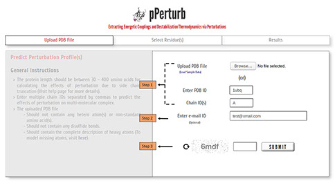Step 1: Upload the PDB file satisfying the considerations specified here (or) enter a valid PDB ID. (Optional) Specify chain ID(s) of the protein to be considered, defaults to first chain entry unless otherwise mentioned.

Note: To upload multimeric structures, enter chain IDs separated by comma.

Step 2: The calculations from the server may take a few minutes depending on the number of residues perturbed (see below). You may provide your e-mail ID (optional) to which the results will be forwarded once the calculations are done.

Step 3: Enter valid CAPTCHA and click on “SUBMIT” to proceed.

Specify Input Parameters

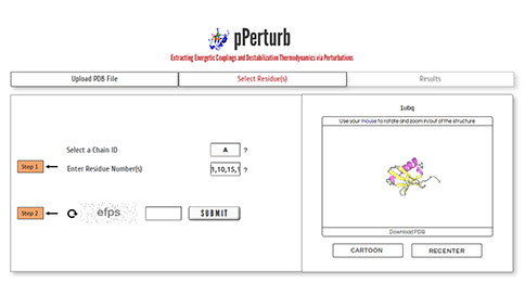
Step 1: Select a chain ID and one or more residue numbers (as in the uploaded PDB file), separated by comma, to predict the perturbation profile due to side-chain truncation.

Note: If you have uploaded multimeric structures, the server estimates the non-isotropic percolation of perturbations into the different subunits.

Step 2: Enter valid CAPTCHA and click on “SUBMIT” to proceed with calculations.

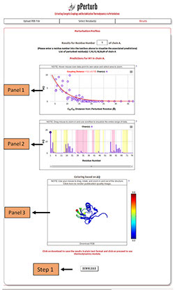Probing the Contact-Network of Residues via Perturbations

Perturbation Profile(s):

Panel 1 shows the distance dependence of the magnitude of perturbation on other residues (ΔQ) from the perturbed site.

Panel 2 depicts ΔQ as a function of residue number (the residue that is perturbed is highlighted by a circle). The shaded regions represent the secondary structure elements in the input PDB file (magenta: α-helix and yellow: β-sheet).

Note: Desired residue can be selected from the list of perturbed residues to visualize the associated predictions.

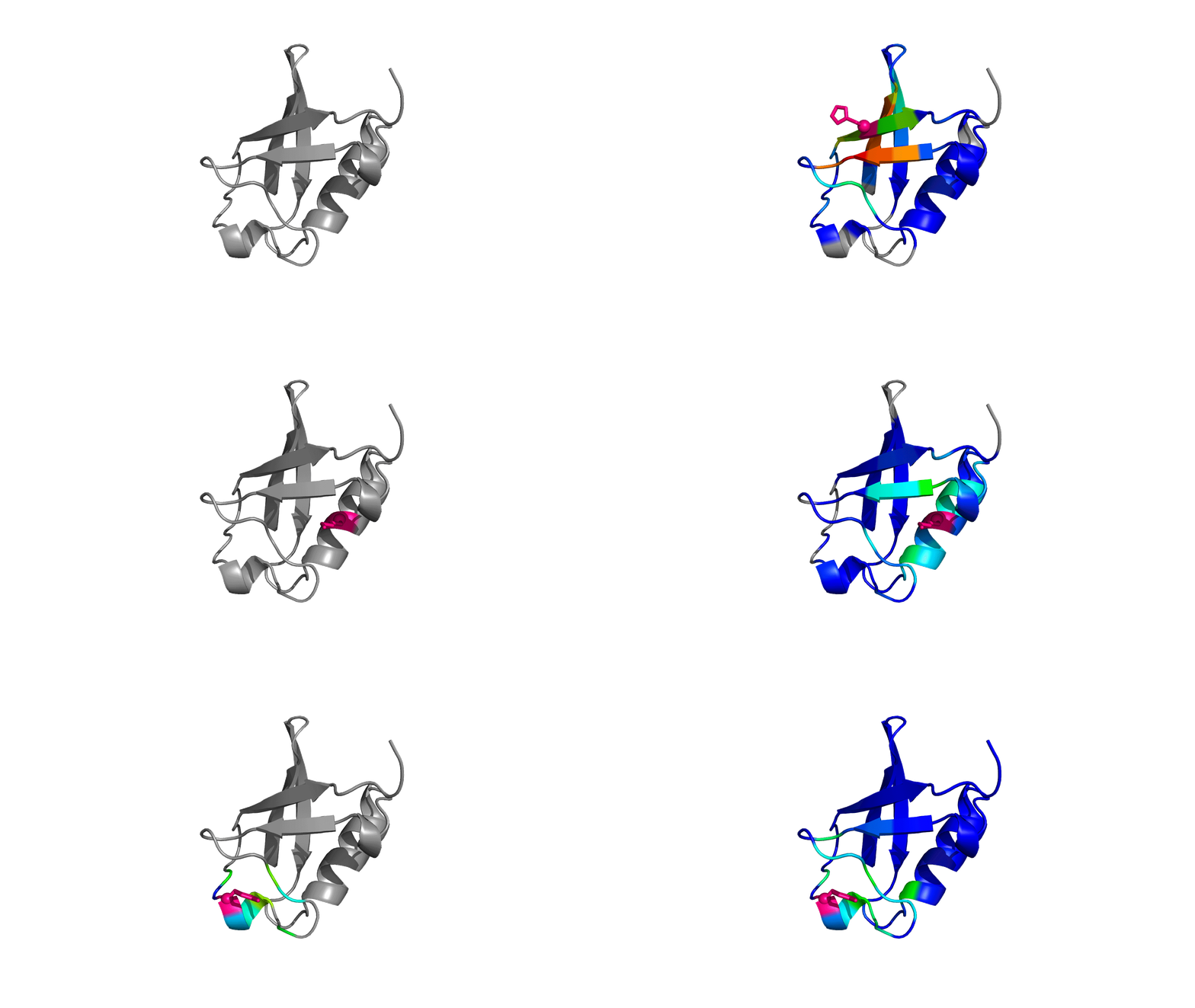
Panel 3: Visualization of the protein structure colored based on ΔQ values. Perturbed residue is shown in ball and stick representation and colored red. Rest of the residues are colored based on ΔQ values following the color spectrum shown adjacent to the panel.

Note: The structure shown in panel 3 can be downloaded as a PDB file and the ∆Q values are mapped on to the temperature factor column. They can be visualized locally in any PDB viewing GUI by coloring the downloaded file based on the B-factor. The users can also generate publication quality images using the link provided in panel 3 (described in detail here).

Step 1: Click on “DOWNLOAD” to save the output data files into your local machine.

B) Generate Interaction-Network Profile

Upload PDB Files

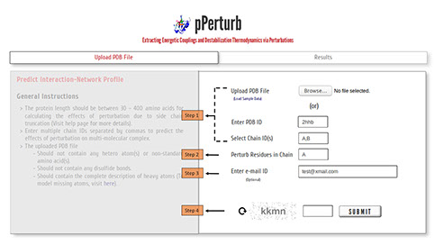Step 1: Upload the PDB file satisfying the considerations specified here (or) enter a valid PDB ID. (Optional) Specify chain ID(s) of the protein to be considered for generating contact map, defaults to first chain entry unless otherwise mentioned.

Step2: Enter a valid chain ID to perturb all the residues iteratively.

Step 3: The calculations from the server may take a few minutes depending on the length of the protein (see below). You may provide your e-mail ID (optional) to which the results will be forwarded once the calculations are done.

Step 4: Enter valid CAPTCHA and click on “SUBMIT” to proceed.

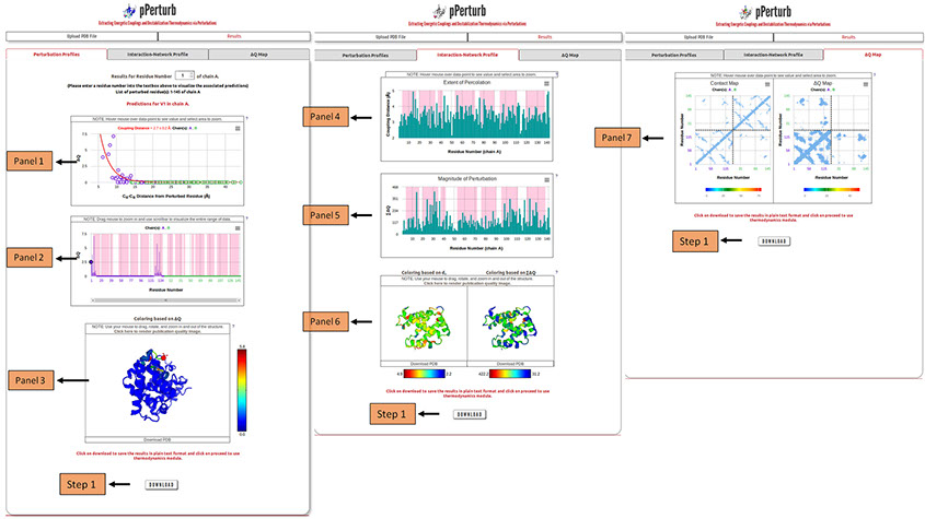
Probing the Contact-Network via Perturbations

Perturbation Profiles (Tab 1): Panel 1 shows the distance dependence of the magnitude of perturbation on other residues (ΔQ) from the perturbed site. Panel 2 depicts ΔQ as a function of residue number (the residue that is perturbed is highlighted by a circle). The shaded regions represent the secondary structure elements in the input PDB file (magenta: α-helix and yellow: β-sheet).

Note: Desired residue can be selected from the list of perturbed residues to visualize the associated predictions.

Panel 3: Visualization of the protein structure colored based on ΔQ values. Perturbed residue is shown in ball and stick representation and colored red. Rest of the residues are colored based on ΔQ values.

Interaction-Network Profile (Tab 2): The extent of percolation is quantified using an exponential fit (as observed in experiments, Rajasekaran N et al, 2017) to the ΔQ vs. Cα-Cα distance profile from the perturbed residue. The interaction-network profile of the protein based on the dC (exponent of the exponential fit) and the total magnitude of perturbation (∑∆Q) is shown in panels 4 and panel 5, respectively.

Panel 6: Visualization of the protein structure colored based on dC and ∑∆Q.

ΔQ-Map (Tab 3): A representation of the contact map and ΔQ map of the protein explicitly depicting the perturbed first and second shell interactions (panel 7).

Step 1: Click on “DOWNLOAD” to save the output data files into your local machine.

Note: To render publication quality image of the displayed protein structure(s), click on the link provided on the top (explained in detail here). Apart from this, the displayed protein structure(s) can also be downloaded as PDB files in which the associated ΔQ/∑∆Q/dC values are mapped onto the temperature factor column. They can be visualized locally in any PDB viewing GUI by coloring the downloaded file based on the B-factor.

C) Compare Interaction-Network Profiles

Upload PDB Files

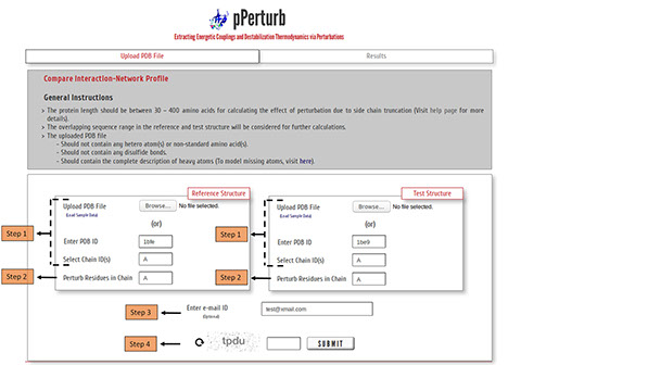Step 1: Upload PDB files of a protein, at two distinct physiological states or ligand-bound/unbound variants, satisfying the considerations mentioned here (or) enter valid PDB IDs to compare the interaction-network profile.

(Optional) Specify chain ID(s) of the protein to be considered for generating contact map, defaults to first chain entry unless otherwise mentioned.

Step2: Enter a valid chain ID to perturb all the residues iteratively.

Step 3: The calculations from the server may take a few minutes depending on the length of the protein (see below). You may provide your e-mail ID (optional) to which the results will be forwarded once the calculations are done.

Step 4: Enter valid CAPTCHA and click on “SUBMIT” to proceed.

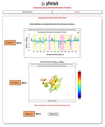Probing the Difference in Interaction-Network via Perturbations

Panel 1 shows the difference in magnitude of contact network, measured as δ = Σ∆Q(T)-Σ∆Q(R). The Σ∆Q represents the total magnitude of the perturbation and the details can be found here.

The Z-score for each residues i is calculated as follows, Zi = (δi - <δ>)/σ(δ). The values can be visualized by hovering mouse over the data points and can be downloaded as a text file following step 1 described below.

Panel 2: Visualization of the protein structure colored based on the differences.

Note: The PDB file can be downloaded and the predicted values are mapped on to the temperature factor column. They can be visualized locally in any PDB viewing GUI by coloring the downloaded file based on the B-factor. The users can also generate publication quality images using the link provided in panel 2 (described in detail here).

Step 1: Click on “DOWNLOAD” to save the output data files into your local machine.

D) Predicting Destabilization Thermodynamics

Upload PDB Files

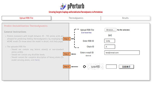Step 1: Upload the PDB file satisfying the considerations specified here (or) enter a valid PDB ID. (Optional) Specify chain ID of the protein to be considered, defaults to first chain entry unless otherwise mentioned.

Step 2: The calculations from the server may take a few minutes depending on the protein length (see below). You may provide your e-mail ID (optional) to which the results will be forwarded once the calculations are done.

Step 3: Enter valid CAPTCHA and click on “SUBMIT” to proceed.

Reproducing Experimental Wild-Type Melting Temperature

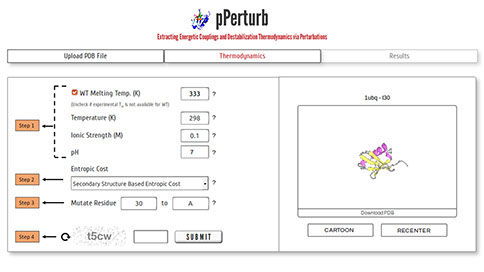Step 1: Specify the experimentally determined melting temperature of the wild type protein. Uncheck the box if experimental data is unavailable and a default value of 333 K will be used. The local stability profile of the protein(s) is predicted at the user-specified temperature, ionic strength and pH.

Step 2: Choose one of the three approaches (refer here) available to assign entropic cost to residues.

Step 3: Enter a valid residue number and amino acid code to simulate side-chain truncation involving uncharged residues.

Note: To mutate (or) introduce charged residues, please visit the pStab web server.

Step 4: Enter valid CAPTCHA and click on “SUBMIT” to proceed with the calculation.

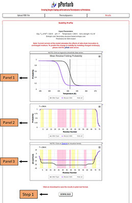Predicting Stability Loss on Side-Chain Truncation

Panel 1: Thermal unfolding profile of WT protein and mutant(s) as a function of temperature. Vertical dashed-line marks the melting temperature of the WT protein.

Panel 2: Residue Folding Probability as a function of residue number. The shaded regions represent the secondary structure elements in the input PDB file (magenta: α-helix and yellow: β-sheet).

Panel 3: Same as panel 3 but for local stability (∆Glocal) as a function of residue number.

Step 1: Click on “DOWNLOAD” to save the corresponding data files into your local machine.

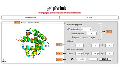Rendering Publication Quality Images

Step 1: Specify the option based on which the image has to be rendered (ΔQ/ dC/ Amplitude).

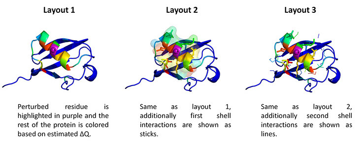
Note: For example, to color based on ΔQ, select a residue from the list of perturbed residues and choose one of the three layouts (explained in following section).

Step 2: Specify the rotation along X-, Y- and/or Z-axis for the required visualization.

Step 3: Specify the size and resolution of the image.

Step 4: Enter valid CAPTCHA and click on “RENDER” to generate high quality image.

Step 5: Click on “DOWNLOAD” to save the PyMOL generated image into your local machine.

Layouts Available to Color Residues Based on Perturbation Profile(s)

Layouts Available to Color Residues while Comparing Interaction-Network Profiles

Structural Perturbation Approach

To understand the effects of residue perturbation on the interaction-network of a protein, we employ a simple structural perturbation protocol that captures the changes in thermodynamic stabilities induced by point mutations within the protein interior (Rajasekaran N et al, 2017). With just the protein contact-map as an input, we reproduce the extent of percolation of perturbations within the structure as observed in network analysis of proteins, molecular dynamics simulations and NMR-observed changes in chemical shifts (Rajasekaran N et al, 2017; Rajasekaran N & Naganathan AN, 2017). Using this rapid protocol that relies on a single structure, we can identify functionally critical sectors, the propagation and dissipation of perturbations within proteins and the higher-order couplings deduced from detailed NMR experiments.

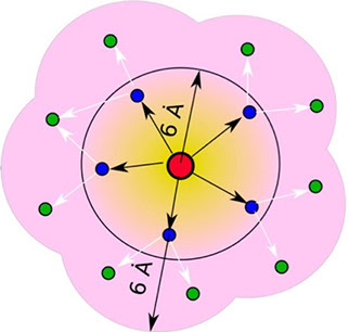
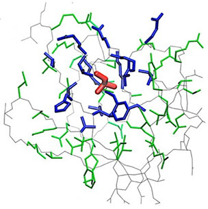
where i is the perturbed residue ( red in figure a & b below), j refers to first shell neighbors ( blue in figure a & b below) and k refers to second shell neighbors ( green in figure a & b below). x1 and x2 are empirical parameters to modulate the extent of perturbation that can be introduced in the first and second shells, respectively, and range from 0 to 1. Different combinations of distance cutoffs and relative destabilizations in the first and second shells (x1 and x2, respectively) were tried in a systematic manner that involved the generation of >100000 unfolding curves (Rajasekaran N et al, 2017). The slope, correlation coefficient, and mean absolute error between the experimental and predicted stability changes were calculated for each of the combinations, and the combination that provides a physically reasonable estimate of all three parameters was chosen.

First shell refers to residues within 6 Å from the perturbed residue and second shell refers to residues within 6 Å from first shell residues. nmut and nWT are the number of heavy atoms present in the perturbed residue (including backbone atoms) before and after mutation. Qx,y is the number of contacts in the contact map between any two residues x and y. All the residues except glycine and alanine are mutated to alanine. Alanine is mutated to glycine and glycine is mutated to a virtual residue with 3 atoms.

a

b

The ΔQ values of each residue, (i.e.) the magnitude of perturbation experienced by each residue, are summed up and plotted as a function of distance from the perturbed residue. The plot is fitted to a exponential function to estimate the exponent (dC) value giving insight into the extent of percolation and Σ∆Q explains the total magnitude of perturbation. All the residues are iteratively perturbed using the above approach to obtain the interaction-network profile of the protein, if specified by the user.

A global ΔQ map is constructed by accumulating all the individual residue-level ΔQ maps and is displayed along with the contact map. Secondary interactions which are not apparent in the contact map can be identified from the global ΔQ map.

Structure-Based Statistical Mechanical Model

To predict the folding thermodynamics of the proteins at a residue-level resolution, we employ an extended version of the simple yet detailed c. The WSME model incorporates multiple energetic terms like vdW interactions, electrostatics, solvation, and residue specific conformational entropy in its energy function. In this model, residues are assumed to sample two sets of conformations: folded (native) and unfolded (non-native) that are assigned the binary variables 1 and 0, respectively thus, leading to a total of 2N structured microstates or conformations for an N-residue protein. In the current version of model, the free energy of each microstate is

where the effective stabilization free-energy of a particular microstate (m, n) (i.e., a string of 1’s between and including m and n) at a temperature T is represented as a sum of van der Waals interactions (EVdW), electrostatic potential (EElec) and solvation free energy (∆Gsolv). ∆S accounts for the entropic cost or penalty for fixing a residue in the native conformation. The details on the model parameters and the values assigned to them by the server can be found here. Further details on the model and equations to calculate the folding probability of residues can be found in the literature (Wako H & Saitô N, 1978; Muñoz V & Eaton WA, 1999; Naganathan AN, 2012).

Errors and Warnings

S.No.	Error	Reason
1	The PDB file does not contain protein molecule(s).	The file uploaded is either empty or does not include information on at least one protein molecule.
2	PDB ID does not exist. Please enter a valid chain ID.	The user has entered an invalid PDB ID.
3	The PDB file contains non-standard (or) post-translationally modified amino acid(s).	The pMutate and Thermodynamics modules do not account for potential stability effects due to non-standard amino acids.
4	The PDB file contains only CA (Cα) atoms. Please upload a PDB file with complete side-chain description.	The server predictions are structure-based and hence require the complete atomic description of every residue (hydrogens are not needed).
5	The protein length is not within the limits (30-400 amino acids) accepted by the web-server.	The server prediction rely on empirical formulations derived from analysis of large scale mutational effects in globular proteins. The empirical relation might not hold true for larger proteins.
7	The PDB file is not complete.	The uploaded protein molecule has missing residues.
8	The PDB file contains multiple amino acids at the same residue position.	Multiple amino acid entries are detected with same residue number.
9	Chain ID does not exist. Please enter a valid chain ID.	The chain ID entered by the user does not exist in the uploaded PDB file (or) the perturbed chain ID is not present in the list of selected chain ID(s).
10	The sequence of the test protein does not match the sequence of the reference protein.	The server compares the interaction-network profile of same protein at two different physiological states.

S.No.	Warning	Reason
1	For this protein, we can generate only the mutational effects and perturbation profile. The protein length should be a monomer with ≤ 150 residues for predicting unfolding curves and local stability maps.	The WSME model, in the cuurent version, does not account for the complex energetic description required for modelling large proteins (refer model description).
2	Considering only the first NMR model from the uploaded PDB file.	The atomic description from the first NMR model is alone considered for predictions.
3	The PDB file contains multiple peptide chains; considering only the first chain.	If the user does not provide a chain ID, the first protein chain from the uploaded file will be considered for further predictions.
4	Residues with missing atomic description are modeled using PyMOL rotamer library.	The residues with missing atoms are modeled using the PyMOL rotamer library. Please verify the fixed pdb file before proceeding with the predictions. Try WHAT IF web server for more detailed modeling of the missing atoms. Caution is required when the backbone atoms are missing.
5	The PDB file contains multiple entries for the same atom(s), considering the first atomic description for each instance.	The first instance of the atomic description is considered for each atom, while the other entries are ignored.
6	Ignoring ligand(s)/hetero-atom(s) in the uploaded PDB file.	Ligand(s) and other hetero atoms present in the PDB file are ignored in the prediction.
7	Residues are renumbered sequentially to remove residue insertion codes.	To maintain consistency in residue numbering, residue insertions are numbered same as that of the N-terminal residue at the insertion point. To provide unique residue identifiers, residues are renumbered sequentially.
8	The length of the protein perturbed in the test case does not match the length of reference protein, considering only the overlapping range of sequence.	The server considers only those residues that are present in both test and reference structures.
9	The PDB file contains disulfide bond(s).	The effects of disulfide bonds are not accounted for in the current version of the web-server.